Chapter 4 Modeling with Multiple Regression
In the previous chapter, you learned about basic regression using either a single numerical or a categorical predictor. But why limit ourselves to using only one variable to inform your explanations/predictions? You will now extend basic regression to multiple regression, which allows for incorporation of more than one explanatory or one predictor variable in your models. You’ll be modeling house prices using a dataset of houses in the Seattle, WA metropolitan area.
Explaining house price with year & size VIDEO
4.1 EDA of relationship
Unfortunately, making 3D scatterplots to perform an EDA is beyond the scope of this course. So instead let’s focus on making standard 2D scatterplots of the relationship between price and the number of bedrooms, keeping an eye out for outliers.
The log10 transformations have been made for you and are saved in house_prices.
- Complete the
ggplot()code to create a scatterplot oflog10_priceoverbedroomsalong with the best-fitting regression line.
library(ggplot2)
library(moderndive)
library(dplyr)
house_prices <- house_prices %>%
  mutate(log10_price = log10(price))
ggplot(data = house_prices, aes(x = bedrooms, y = log10_price)) +
  geom_point() +
  labs(x = "Number of bedrooms", y = "log10 price") +
  geom_smooth(method = "lm", se = FALSE) +
  theme_bw()
There is one house that has 33 bedrooms. While this could truly be the case, given the number of bedrooms in the other houses, this is probably an outlier.
Remove this outlier using
filter()to recreate the plot.
house_prices %>%
  filter(bedrooms < 33) %>%
  ggplot(aes(x = bedrooms, y = log10_price)) +
  geom_point() +
  labs(x = "Number of bedrooms", y = "log10 price") +
  geom_smooth(method = "lm", se = FALSE) +
  theme_bw()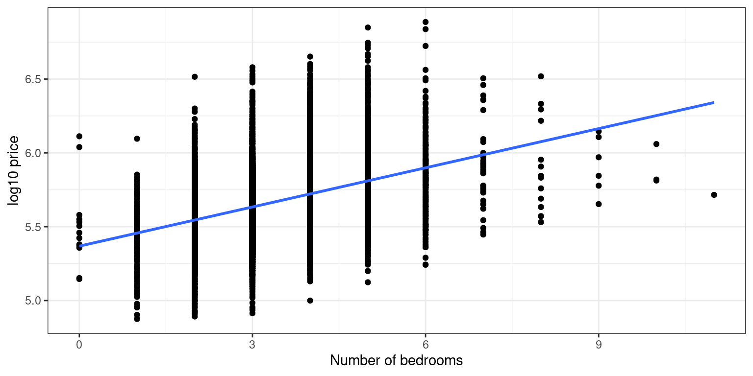
Another important reason to perform EDA is to discard any potential outliers that are likely data entry errors. In our case, after removing an outlier, you can see a clear positive relationship between the number of bedrooms and price, as one would expect.
4.2 Fitting a regression
house_prices, which is available in your environment, has the log base 10 transformed variables included and the outlier house with 33 bedrooms removed. Let’s fit a multiple regression model of price as a function of size and the number of bedrooms and generate the regression table. In this exercise, you will first fit the model, and based on the regression table, in the second part, you will answer the following question:
Which of these interpretations of the slope coefficent for bedrooms is correct?
# Creating and munging the data set
library(moderndive)
house_prices %>%
  mutate(log10_price = log10(price), log10_size = log10(sqft_living)) %>%
  filter(bedrooms < 33) -> house_prices
Fit a linear model lm with
log_10priceas a function oflog10_sizeandbedrooms.Print the regression table.
# Fit model
model_price_2 <- lm(log10_price ~ log10_size + bedrooms,
                    data = house_prices)
# Get regression table
get_regression_table(model_price_2)# A tibble: 3 × 7
term estimate std_error statistic p_value lower_ci upper_ci
<chr> <dbl> <dbl> <dbl> <dbl> <dbl> <dbl>
1 intercept 2.69 0.023 116. 0 2.65 2.74
2 log10_size 0.941 0.008 118. 0 0.925 0.957
3 bedrooms -0.033 0.002 -20.5 0 -0.036 -0.03 Which of these interpretations of the slope coefficent for bedrooms is correct?
Every extra bedroom is associated with a decrease of on average 0.033 in
log10_price.Accounting for
log10_size, every extra bedroom is associated with a decrease of on average 0.033 inlog10_price.
Note: In this multiple regression setting, the associated effect of any variable must be viewed in light of the other variables in the model. In our case, accounting for the size of the house reverses the relationship of the number of bedrooms and price from positive to negative!
Predicting house price using year & size VIDEO
4.3 Making predictions using size and bedrooms
Say you want to predict the price of a house using this model and you know it has:
1000 square feet of lining space, and
3 bedrooms
What is your prediction both in log10 dollars and then dollars?
The regression model from the previous exercise is available in your workspace as model_price_2.
get_regression_table(model_price_2)# A tibble: 3 × 7
term estimate std_error statistic p_value lower_ci upper_ci
<chr> <dbl> <dbl> <dbl> <dbl> <dbl> <dbl>
1 intercept 2.69 0.023 116. 0 2.65 2.74
2 log10_size 0.941 0.008 118. 0 0.925 0.957
3 bedrooms -0.033 0.002 -20.5 0 -0.036 -0.03 - Using the fitted values of the intercept and slopes from the regression table, predict this house’s price in log10 dollars.
# Make prediction in log10 dollars
2.69 + 0.941 * 3 - 0.033 * 3
[1] 5.414*Predict this houses’s pirce in dollars.
# Make prediction dollars
10^(2.69 + 0.941 * log10(1000) - 0.033 * 3)
[1] 259417.9Using the values in the regression table you can make predictions of house prices! In this case, your prediction is about 260,000. Let’s now apply this procedure to all 21k houses!
4.4 Interpreting residuals
Let’s automate this process for all 21K rows in house_prices
to obtain residuals, which you’ll use to compute the sum of squared residuals: a measure of the lack of fit of a model.
- Apply the relevant wrapper function to automate computation of fitted/predicted values and hence also residuals for all 21K houses using
model_price_2.
get_regression_points(model_price_2)# A tibble: 21,612 × 6
ID log10_price log10_size bedrooms log10_price_hat residual
<int> <dbl> <dbl> <int> <dbl> <dbl>
1 1 5.35 3.07 3 5.48 -0.138
2 2 5.73 3.41 3 5.80 -0.071
3 3 5.26 2.89 2 5.34 -0.087
4 4 5.78 3.29 4 5.66 0.123
5 5 5.71 3.22 3 5.63 0.079
6 6 6.09 3.73 4 6.07 0.014
7 7 5.41 3.23 3 5.64 -0.226
8 8 5.46 3.02 3 5.44 0.025
9 9 5.36 3.25 3 5.65 -0.291
10 10 5.51 3.28 3 5.68 -0.167
# … with 21,602 more rows- Compute the sum of squared residuals using dplyr commands.
# Automate prediction and residual computation
get_regression_points(model_price_2) %>%
  mutate(sq_residuals = residual^2) %>%
  summarize(sum_sq_residuals = sum(sq_residuals))
# A tibble: 1 × 1
sum_sq_residuals
<dbl>
1 604.Which of these statement about residuals in incorrect?
The residual is the observed outcome variable minus the predicted variable.
Residuals are leftover points not accounted for in the our regression model.
They can be thought of as prediction errors.
They can be thought of as the lack-of-fit of the predictions to truth.
Note: Residual does not suggest ‘leftovers,’ but not in the sense that they are leftover points.
Explaining house price with size and condition VIDEO
4.5 Parallel slopes model
Let’s now fit a “parallel slopes” model with the numerical explanatory/predictor variable log10_size and the categorical, in this case binary, variable waterfront. The visualization corresponding to this model is below:
# A tibble: 3 × 7
  term           estimate std_error statistic p_value lower_ci upper_ci
  <chr>             <dbl>     <dbl>     <dbl>   <dbl>    <dbl>    <dbl>
1 intercept         2.96      0.02      146.        0    2.92     3.00
2 waterfrontTRUE    0.322     0.013      24.5       0    0.296    0.348
3 log10_size        0.825     0.006     134.        0    0.813    0.837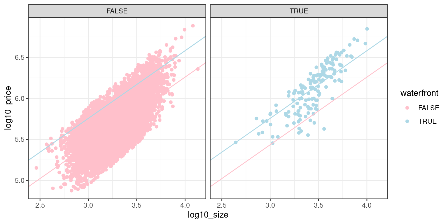
- Fit a multiple regression of
log10_priceusinglog10_sizeandwaterfrontas the predictors. Recall that the data frame that contains these variables ishouse_prices.
# Fit model
model_price_4 <- lm(log10_price ~ log10_size + waterfront,
                    data = house_prices)

# Get regression table
get_regression_table(model_price_4)
# A tibble: 3 × 7
term estimate std_error statistic p_value lower_ci upper_ci
<chr> <dbl> <dbl> <dbl> <dbl> <dbl> <dbl>
1 intercept 2.96 0.02 146. 0 2.92 3.00
2 log10_size 0.825 0.006 134. 0 0.813 0.837
3 waterfrontTRUE 0.322 0.013 24.5 0 0.296 0.348Notice how the regression table has three rows: intercept, the slope for log10_size, and an offset for houses that do have a waterfront.
Let’s interpret the values in the regression table for the parallel slopes model you just fit. Run get_regression_table(model_price_4) in the console to view the regression table again. The visualization for this model is above. Which of these interpretations is incorrect?
_ The intercept for houses with a view of the waterfront is 3.282.
All houses are assumed to have the same slope between
log10_price&log10_size.The intercept for houses without a view of the waterfront is 2.96.
The intercept for houses with a view of the waterfront is 0.322.
Predicting house price using size & condition VIDEO
4.6 Making predictions using size and waterfront
Using your model for log10_price as a function of log10_size and the binary variable waterfront, let’s make some predictions! Say you have the two following “new” houses, what would you predict their prices to be in dollars?
House A: log10_size = 2.9 that has a view of the waterfront
House B: log10_size = 3.1 that does not have a view of the waterfront
ggplot(data = house_prices, aes(x = log10_size, y = log10_price, color = waterfront)) +
  geom_point() +
  facet_wrap(vars(waterfront)) +
  geom_abline(intercept = 2.96, slope = 0.825, color = "red") +
  geom_abline(intercept = 2.96 + 0.322, slope = 0.825, color = "blue") +
  geom_vline(xintercept = 2.9, color = "red") +
  geom_vline(xintercept = 3.1, color = "blue") +
  scale_color_manual(values = c("pink", "lightblue")) +
  theme_bw()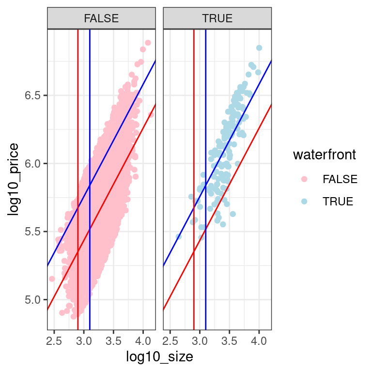
get_regression_table(model_price_4)# A tibble: 3 × 7
term estimate std_error statistic p_value lower_ci upper_ci
<chr> <dbl> <dbl> <dbl> <dbl> <dbl> <dbl>
1 intercept 2.96 0.02 146. 0 2.92 3.00
2 log10_size 0.825 0.006 134. 0 0.813 0.837
3 waterfrontTRUE 0.322 0.013 24.5 0 0.296 0.348- Compute the predicted prices for both houses. First you’ll use an equation based on values in the regression table (above) to get a predicted value in log10 dollars, then raise 10 to this predicted value to get a predicted value in dollars.
# Prediction for House A
10^get_regression_points(model_price_4, newdata = data.frame(log10_size = 2.9, waterfront = TRUE))[4]
log10_price_hat
1 472063# 10^5.67
# OR
10^predict(model_price_4, newdata = data.frame(log10_size = 2.9, waterfront = TRUE)) 1
471621.4 # OR
10^(coefficients(model_price_4)[1] + coefficients(model_price_4)[2]*2.9 + coefficients(model_price_4)[3])(Intercept)
471621.4 # Prediction for House B
10^get_regression_points(model_price_4, newdata = data.frame(log10_size = 3.1, waterfront = FALSE))[4] log10_price_hat
1 328095.3# 10^5.52
# OR
10^predict(model_price_4, newdata = data.frame(log10_size = 3.1, waterfront = FALSE)) 1
328442 10^(2.96 + 0.825 * 3.1)[1] 329230.5# OR
10^(coefficients(model_price_4)[1] + coefficients(model_price_4)[2]*3.1 + coefficients(model_price_4)[3]*0)(Intercept)
328442 4.7 Automating predicing on “new” houses
Let’s now repeat what you did in the last exercise, but in an automated fashion assuming the information on these “new” houses is saved in a dataframe.
Your model for log10_price as a function of log10_size and the binary variable waterfront (model_price_4) is available in your workspace, and so is new_houses_2, a dataframe with data on 2 new houses. While not so beneficial with only 2 “new” houses, this will save a lot of work if you had 2000 “new” houses.
new_houses_2 <- data.frame(log10_size = c(2.9, 3.1), waterfront = c(TRUE, FALSE))
new_houses_2
log10_size waterfront
1 2.9 TRUE
2 3.1 FALSE- Apply
get_regression_points()as you would normally, but with thenewdataargument set to our two “new” houses. This returns predicted values for just those houses.
get_regression_points(model_price_4, newdata = new_houses_2)# A tibble: 2 × 4
ID log10_size waterfront log10_price_hat
<int> <dbl> <lgl> <dbl>
1 1 2.9 TRUE 5.67
2 2 3.1 FALSE 5.52- Now take these two predictions in
log10_price_hatand return a new column,price_hat, consisting of fitted price in dollars.
# Get predictions price_hat in dollars on "new" houses
get_regression_points(model_price_4, newdata = new_houses_2) %>%
  mutate(price_hat = 10^log10_price_hat)
# A tibble: 2 × 5
ID log10_size waterfront log10_price_hat price_hat
<int> <dbl> <lgl> <dbl> <dbl>
1 1 2.9 TRUE 5.67 472063.
2 2 3.1 FALSE 5.52 328095.