Chapter 2 Introduction to Modeling
This chapter will introduce you to some background theory and terminology for modeling, in particular, the general modeling framework, the difference between modeling for explanation and modeling for prediction, and the modeling problem. Furthermore, you’ll start performing your first exploratory data analysis, a crucial first step before any formal modeling.
Background on modeling for explanation VIDEO
2.1 Exploratory visualization of age
Let’s perform an exploratory data analysis (EDA) of the numerical explanatory variable age. You should always perform an exploratory analysis of your variables before any formal modeling. This will give you a sense of your variable’s distributions, any outliers, and any patterns that might be useful when constructing your eventual model.
Use the
evalsdata set from themoderndivepackage along withggplot2to create a histogram ofagewith bins in 5 year increments.Label the
xaxis withageand theyaxis with count.
# Load packages
library(moderndive)
library(ggplot2)

# Plot the histogram
ggplot(evals, aes(x = age)) +
  geom_histogram(binwidth = 5) +
  labs(x = "age", y = "count")
2.2 Numerical summaries of age
Let’s continue our exploratory data analysis of the numerical explanatory variable age by computing summary statistics. Summary statistics take many values and summarize them with a single value. Let’s compute three such values using dplyr data wrangling: mean (AKA the average), the median (the middle value), and the standard deviation (a measure of spread/variation).
- Calculate the mean, median, and standard deviation of
age.
# Load packages
library(moderndive)
library(dplyr)

# Compute summary stats
evals %>%
  summarize(mean_age = mean(age),
            median_age = median(age),
            sd_age = sd(age))
# A tibble: 1 × 3
mean_age median_age sd_age
<dbl> <int> <dbl>
1 48.4 48 9.80Background on modeling for prediction VIDEO
2.3 Exploratory visualization of house size
Let’s create an exploratory visualization of the predictor variable reflecting the size of houses: sqft_living the square footage of living space where 1 sq.foot \(\approx\) 0.1 sq.meter.
After plotting the histogram, what can you say about the distribution of the variable sqft_living?
Create a histogram of
sqft_livingusing thehouse_pricesdata set from themoderndivepackage.Label thexaxis with“Size (sq.feet)”and theyaxis with“count”`.
# Plot the histogram
ggplot(house_prices, aes(x = sqft_living)) +
  geom_histogram() +
  labs(x = "Size (sq.feet)", y = "count") +
  theme_bw()
`stat_bin()` using `bins = 30`. Pick better value with `binwidth`.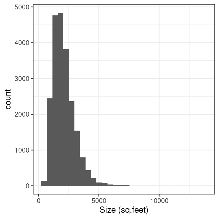
2.4 Log10 transformation of house size
You just saw that the predictor variable sqft_living is right-skewed and hence a log base 10 transformation is warranted to unskew it. Just as we transformed the outcome variable price to create log10_price in the video, let’s do the same for sqft_living.
- Using the
mutate()function fromdplyr, create a new columnlog10_sizeand assign it tohouse_prices_2by applying alog10()transformation tosqft_living.
# Add log10_size
house_prices_2 <- house_prices %>%
mutate(log10_size = log10(sqft_living))- Visualize the effect of the
log10()transformation by creating a histogram of the new variablelog10_size.
# Plot the histogram
ggplot(house_prices_2, aes(x = log10_size)) +
  geom_histogram() +
  labs(x = "log10 size", y = "count") +
  theme_bw()
`stat_bin()` using `bins = 30`. Pick better value with `binwidth`.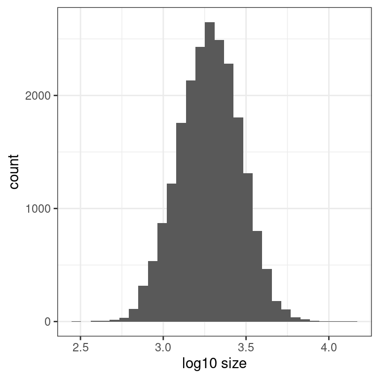
Notice how the distribution is much less skewed. Going forward, you will use this new transformed variable to represent the size of houses.
The modeling problem for explanation VIDEO
2.5 EDA of relationship of teaching & “beauty” scores
The researchers in the UT Austin created a “beauty score” by asking a panel of 6 students to rate the “beauty” of all 463 instructors. They were interested in studying any possible impact of “beauty” of teaching evaluation scores. Let’s do an EDA of this variable and its relationship with teaching score. The data are stored in evals.
From now on, assume that ggplot2, dplyr, and moderndive are all available in your workspace unless you’re told otherwise.
- Create a histogram of
bty_avg“beauty scores” with bins of size 0.5.
### Plot the histogram
ggplot(evals, aes(x = bty_avg)) +
  geom_histogram(color = "black", fill = "red", binwidth = 0.5) +
  labs(x = "Beauty score", y = "count") +
  theme_bw()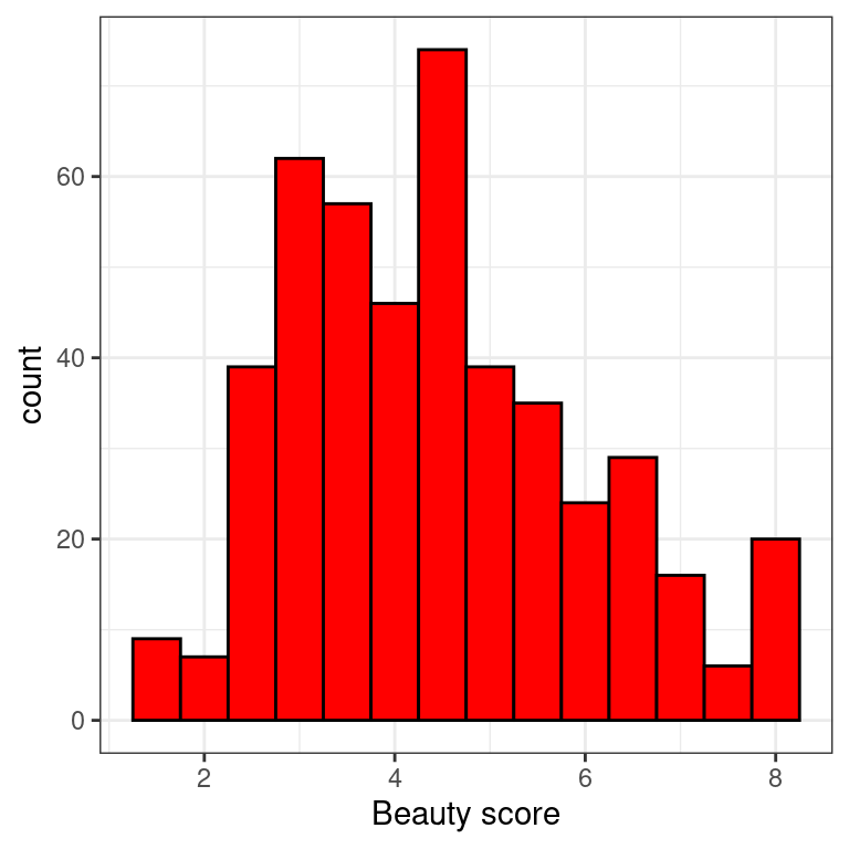
- Create a scatterplot with the outcome variable
scoreon the y-axis and the explanatory variablebty_avgon the x-axis.
# Scatterplot
ggplot(evals, aes(x = bty_avg, y = score)) +
  geom_point() +
  labs(x = "beauty score", y = "teaching score") +
  theme_bw()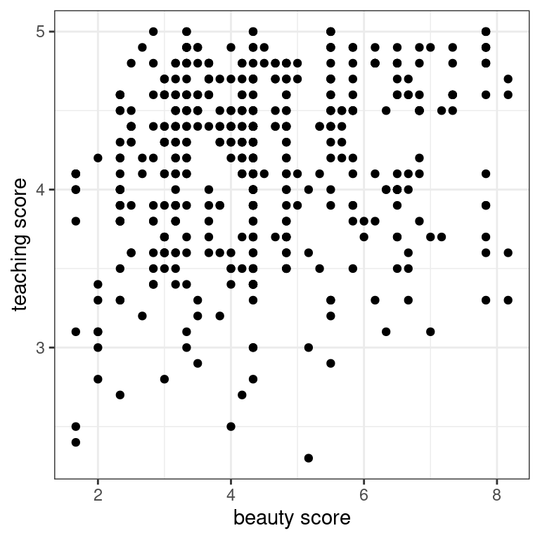
- Let’s now investigate if this plot suffers from overplotting, whereby points are stacked perfectly on top of each other, obscuring the number of points involved. You can do this by jittering the points. Update the code accordingly!
# Jitter plot
ggplot(evals, aes(x = bty_avg, y = score)) +
  geom_jitter() +
  labs(x = "beauty score", y = "teaching score") +
  theme_bw()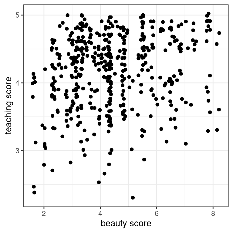
It seems the original scatterplot did suffer from overplotting since the jittered scatterplot reveals many originally hidden points. Most bty_avg scores range from 2-8, with 5 being about the center.
2.6 Correlation between teaching and “beauty” scores
Let’s numerically summarize the relationship between teaching score and beauty score bty_avg using the correlation coefficient. Based on this, what can you say about the relationship between these two variables?
- Compute the correlation coefficient of
scoreandbty_avg.
# Compute correlation
evals %>%
  summarize(correlation = cor(score, bty_avg))
# A tibble: 1 × 1
correlation
<dbl>
1 0.187Highlight the appropriate answer:
scoreandbty_avgare strongly negatively associated.scoreandbty_avgare weakly negatively associated.scoreandbty_avgare weakly positively associated.scoreandbty_avgare strongly positively associated.
While there seems to be a positive relationship, 0.187 is still a long ways from 1, so the correlation is only weakly positive.
The modeling problem for prediction VIDEO
2.7 EDA of relationship of house price and waterfront
Let’s now perform an exploratory data analysis of the relationship between log10_price, the log base 10 house price, and the binary variable waterfront. Let’s look at the raw values of waterfront and then visualize their relationship.
The column log10_price has been added for you in the house_prices dataset.
house_prices %>%
mutate(log10_price = log10(price)) -> house_prices- Use
glimpse()to view the structure of only two columns:log10_priceandwaterfront.
# View the structure of log10_price and waterfront
house_prices %>%
  select(log10_price, waterfront) %>%
  glimpse()
Rows: 21,613
Columns: 2
$ log10_price <dbl> 5.346157, 5.730782, 5.255273, 5.781037, 5.707570, 6.088136…
$ waterfront <lgl> FALSE, FALSE, FALSE, FALSE, FALSE, FALSE, FALSE, FALSE, FA…- Visualize the relationship between
waterfrontandlog10_priceusing an appropriategeom_*function. Remember thatwaterfrontis categorical.
# Plot
ggplot(house_prices, aes(x = waterfront, y = log10_price)) +
  geom_boxplot() +
labs(x = "waterfront", y = "log10 price") 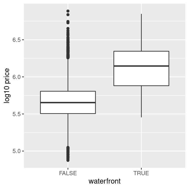
Look at that boxplot! Houses that have a view of the waterfront tend to be MUCH more expensive as evidenced by the much higher log10 prices!
2.8 Predicting house price with waterfront
You just saw that houses with a view of the waterfront tend to be much more expensive. But by how much? Let’s compute group means of log10_price, convert them back to dollar units, and compare!
- Return both the mean of
log10_priceand the count of houses in each level ofwaterfront
# Calculate stats
house_prices %>%
  group_by(waterfront) %>%
  summarize(mean_log10_price = mean(log10_price), n = n())
# A tibble: 2 × 3
waterfront mean_log10_price n
<lgl> <dbl> <int>
1 FALSE 5.66 21450
2 TRUE 6.12 163- Using these group means for
log10_price, return “good” predicted house prices in the original units of US dollars.
# Prediction of price for houses with view
10^(6.12)
[1] 1318257# Prediction of price for houses without view
10^(5.66)[1] 457088.2Most houses don’t have a view of the waterfront (\(n = 21,450\)), but those that do (\(n = 163\)) have a MUCH higher predicted price. Look at that difference! 457,088 versus 1,318,257! In the upcoming Chapter 2 on basic regression, we’ll build on such intuition and construct our first formal explanatory and predictive models using basic regression!